Make Figure 1
Last updated: 2022-10-23
Checks: 7 0
Knit directory: Code/
This reproducible R Markdown analysis was created with workflowr (version 1.7.0). The Checks tab describes the reproducibility checks that were applied when the results were created. The Past versions tab lists the development history.
Great! Since the R Markdown file has been committed to the Git repository, you know the exact version of the code that produced these results.
Great job! The global environment was empty. Objects defined in the global environment can affect the analysis in your R Markdown file in unknown ways. For reproduciblity it’s best to always run the code in an empty environment.
The command set.seed(20211230) was run prior to running
the code in the R Markdown file. Setting a seed ensures that any results
that rely on randomness, e.g. subsampling or permutations, are
reproducible.
Great job! Recording the operating system, R version, and package versions is critical for reproducibility.
Nice! There were no cached chunks for this analysis, so you can be confident that you successfully produced the results during this run.
Great job! Using relative paths to the files within your workflowr project makes it easier to run your code on other machines.
Great! You are using Git for version control. Tracking code development and connecting the code version to the results is critical for reproducibility.
The results in this page were generated with repository version bbb4c58. See the Past versions tab to see a history of the changes made to the R Markdown and HTML files.
Note that you need to be careful to ensure that all relevant files for
the analysis have been committed to Git prior to generating the results
(you can use wflow_publish or
wflow_git_commit). workflowr only checks the R Markdown
file, but you know if there are other scripts or data files that it
depends on. Below is the status of the Git repository when the results
were generated:
Ignored files:
    Ignored:    .DS_Store
    Ignored:    .Rhistory
    Ignored:    .Rproj.user/
    Ignored:    Flexibility Comparisons.nb.html
    Ignored:    Main.nb.html
    Ignored:    PGLS.FullData.nb.html
    Ignored:    PGLSforeachMeasFeature.nb.html
    Ignored:    PGLSwithPCA_Dims.nb.html
    Ignored:    PreppedVertMeas.nb.html
    Ignored:    ProcessCymatogasterFiles.nb.html
    Ignored:    ProcessFCSVfiles.nb.html
    Ignored:    TestingHabitatwithFriedmanData.nb.html
    Ignored:    Trilok_tree.nb.html
    Ignored:    VertLM.nb.html
    Ignored:    VertMeasLDA_Attempt.nb.html
    Ignored:    VertPGLS.nb.html
    Ignored:    VertPairs.nb.html
    Ignored:    analysis/.DS_Store
    Ignored:    analysis/.Rhistory
    Ignored:    analysis/02-CheckSpeciesMatch.nb.html
    Ignored:    analysis/10-VertLM.nb.html
    Ignored:    analysis/12-VertPGLS2.nb.html
    Ignored:    analysis/13-VertPGLS-MANOVA40.nb.html
    Ignored:    analysis/13-VertPGLS-MANOVA90.nb.html
    Ignored:    analysis/14-VertPGLS-MANOVA40.nb.html
    Ignored:    analysis/20-plot_phylogeny.nb.html
    Ignored:    analysis/21-plot_fits_and_summary.nb.html
    Ignored:    analysis/CheckSpeciesMatch.nb.html
    Ignored:    caper_test.nb.html
    Ignored:    data/.DS_Store
    Ignored:    ggtree_attempt.nb.html
    Ignored:    output/.DS_Store
    Ignored:    plot_example_data.nb.html
    Ignored:    plot_fits_and_summary.nb.html
    Ignored:    plot_phylogeny.nb.html
    Ignored:    summarize_vert_meas.nb.html
    Ignored:    test_phylogeny.nb.html
    Ignored:    test_vertebraspace.nb.html
    Ignored:    vert_evol.Rproj

Untracked files:
    Untracked:  Archive.zip
    Untracked:  Main.html
    Untracked:  ProcessFCSVfiles.Rmd
    Untracked:  VertPGLS.html
    Untracked:  analysis/13-VertPGLS-MANOVA90.Rmd
    Untracked:  analysis/14-VertPGLS-MANOVA40.Rmd
    Untracked:  data/actinopt_12k_raxml.tre.xz
    Untracked:  gg_saver.R
    Untracked:  output/BodyDistribution.pdf
    Untracked:  output/MasterVert_Measurements.csv
    Untracked:  output/anova_table.rtf
    Untracked:  output/anovatabs.csv
    Untracked:  output/effectsizes.csv
    Untracked:  output/fineness.pdf
    Untracked:  output/habitatvals.csv
    Untracked:  output/manova_table.rtf
    Untracked:  output/mean_d_alphaPos_CBL.pdf
    Untracked:  output/mean_params.pdf
    Untracked:  output/pair_plot.pdf
    Untracked:  output/phylogeny_families.pdf
    Untracked:  output/plot_example_data_figure.pdf
    Untracked:  output/predvals.Rds
    Untracked:  output/stats_table.rtf
    Untracked:  output/vertdata_show_species.csv
    Untracked:  output/vertdata_summary_species.csv
    Untracked:  output/vertshape.pdf
    Untracked:  plot_fits_and_summary.Rmd
    Untracked:  summarize_vert_meas.html
    Untracked:  testtree.csv
    Untracked:  vert_tree.csv

Unstaged changes:
    Deleted:    .Rprofile
    Modified:   analysis/index.Rmd
    Modified:   data/MasterVert_Measurements.csv
    Modified:   output/MasterVert_Measurements_Matched.csv
    Modified:   output/vert_tree.rds
    Modified:   output/vertdata_centered.csv
    Modified:   output/vertdata_summary.csv
    Deleted:    renv.lock
    Deleted:    renv/.gitignore
    Deleted:    renv/activate.R
    Deleted:    renv/settings.dcf
Note that any generated files, e.g. HTML, png, CSS, etc., are not included in this status report because it is ok for generated content to have uncommitted changes.
These are the previous versions of the repository in which changes were
made to the R Markdown (analysis/20-plot_phylogeny.Rmd) and
HTML (docs/20-plot_phylogeny.html) files. If you’ve
configured a remote Git repository (see ?wflow_git_remote),
click on the hyperlinks in the table below to view the files as they
were in that past version.
| File | Version | Author | Date | Message |
|---|---|---|---|---|
| Rmd | bbb4c58 | Eric Tytell | 2022-10-23 | Final analysis scripts |
| Rmd | 65e217e | Eric Tytell | 2022-09-16 | Updated code |
| Rmd | 8b12300 | Eric Tytell | 2022-09-06 | Assorted updates |
| html | 5e4be8c | Eric Tytell | 2022-04-11 | Build site. |
| Rmd | 23908bd | Eric Tytell | 2021-12-30 | Test site build again |
| Rmd | edeae3c | Eric Tytell | 2021-12-30 | Rename notebooks to indicate order |
library(tidyverse)── Attaching packages ─────────────────────────────────────── tidyverse 1.3.2 ──
✔ ggplot2 3.3.6 ✔ purrr 0.3.4
✔ tibble 3.1.8 ✔ dplyr 1.0.9
✔ tidyr 1.2.0 ✔ stringr 1.4.1
✔ readr 2.1.2 ✔ forcats 0.5.2
── Conflicts ────────────────────────────────────────── tidyverse_conflicts() ──
✖ dplyr::filter() masks stats::filter()
✖ dplyr::lag() masks stats::lag()library(ggbeeswarm)
library(phytools)Loading required package: ape
Loading required package: maps
Attaching package: 'maps'
The following object is masked from 'package:purrr':
maplibrary(patchwork)
library(here)here() starts at /Users/etytel01/Documents/Vertebrae/Codelibrary(ggtree)Warning: package 'ggtree' was built under R version 4.2.1ggtree v3.4.2 For help: https://yulab-smu.top/treedata-book/
If you use the ggtree package suite in published research, please cite
the appropriate paper(s):
Guangchuang Yu, David Smith, Huachen Zhu, Yi Guan, Tommy Tsan-Yuk Lam.
ggtree: an R package for visualization and annotation of phylogenetic
trees with their covariates and other associated data. Methods in
Ecology and Evolution. 2017, 8(1):28-36. doi:10.1111/2041-210X.12628
G Yu. Data Integration, Manipulation and Visualization of Phylogenetic
Trees (1st ed.). Chapman and Hall/CRC. 2022. ISBN: 9781032233574
LG Wang, TTY Lam, S Xu, Z Dai, L Zhou, T Feng, P Guo, CW Dunn, BR
Jones, T Bradley, H Zhu, Y Guan, Y Jiang, G Yu. treeio: an R package
for phylogenetic tree input and output with richly annotated and
associated data. Molecular Biology and Evolution. 2020, 37(2):599-603.
doi: 10.1093/molbev/msz240
Attaching package: 'ggtree'
The following object is masked from 'package:ape':
rotate
The following object is masked from 'package:tidyr':
expandlibrary(plotly)
Attaching package: 'plotly'

The following object is masked from 'package:ggplot2':

    last_plot

The following object is masked from 'package:stats':

    filter

The following object is masked from 'package:graphics':

    layout
Figure 1
For this figure, we need to identify three species from the three habitat classes that have clearly different vertebrae.
vertdata <- read_csv(here('output/vertdata_summary_species.csv'))Rows: 82 Columns: 46
── Column specification ────────────────────────────────────────────────────────
Delimiter: ","
chr (7): Species, Habitat, Water_Type, MatchSpecies, alltaxon, Order, Family
dbl (39): Indiv, fineness, CBL_med, CBL_max, CBL_mn, d_med, d_max, d_mn, alp...
ℹ Use `spec()` to retrieve the full column specification for this data.
ℹ Specify the column types or set `show_col_types = FALSE` to quiet this message.plot_ly(data = vertdata, type = "scatter", mode = "markers") %>%
add_trace(x = ~Habitat, y = ~d_med, type = "box",
text = ~Species, hoverinfo = "text",
boxpoints = "all", jitter = 0.2)Warning: Can't display both discrete & non-discrete data on same axisWarning: 'box' objects don't have these attributes: 'mode'
Valid attributes include:
'alignmentgroup', 'boxmean', 'boxpoints', 'customdata', 'customdatasrc', 'dx', 'dy', 'fillcolor', 'hoverinfo', 'hoverinfosrc', 'hoverlabel', 'hoveron', 'hovertemplate', 'hovertemplatesrc', 'hovertext', 'hovertextsrc', 'ids', 'idssrc', 'jitter', 'legendgroup', 'legendgrouptitle', 'legendrank', 'line', 'lowerfence', 'lowerfencesrc', 'marker', 'mean', 'meansrc', 'median', 'mediansrc', 'meta', 'metasrc', 'name', 'notched', 'notchspan', 'notchspansrc', 'notchwidth', 'offsetgroup', 'opacity', 'orientation', 'pointpos', 'q1', 'q1src', 'q3', 'q3src', 'quartilemethod', 'sd', 'sdsrc', 'selected', 'selectedpoints', 'showlegend', 'stream', 'text', 'textsrc', 'transforms', 'type', 'uid', 'uirevision', 'unselected', 'upperfence', 'upperfencesrc', 'visible', 'whiskerwidth', 'width', 'x', 'x0', 'xaxis', 'xcalendar', 'xhoverformat', 'xperiod', 'xperiod0', 'xperiodalignment', 'xsrc', 'y', 'y0', 'yaxis', 'ycalendar', 'yhoverformat', 'yperiod', 'yperiod0', 'yperiodalignment', 'ysrc', 'key', 'set', 'frame', 'transforms', '_isNestedKey', '_isSimpleKey', '_isGraticule', '_bbox'A tibble: 12 × 47
Species Indiv Habitat Water…¹ Match…² allta…³ Order Family finen…⁴
CBL_med
Choose example species close to the median for their group:
- benthic: Barbichthys laevis (Sucker barb) or Myoxocephalus polyacanthocephalus (Sculpin)
- demersal: Poecilia reticulata (Guppy)
- pelagic: Sphyraena sphyraena (Barracuda)
We’ll use the sculpin as an example benthic species, because we have good histology data for it.
examplespecies <- list("Myoxocephalus_polyacanthocephalus",
                    "Anoplarchus_purpurescens",
                    "Cymatogaster_aggregata")
verttree <- readRDS(here('output/vert_tree.rds'))vertdata %>%
filter(Species %in% examplespecies)# A tibble: 3 × 46
Species Indiv Habitat Water…¹ Match…² allta…³ Order Family finen…⁴ CBL_med
<chr> <dbl> <chr> <chr> <chr> <chr> <chr> <chr> <dbl> <dbl>
1 Anoplarchu… 1 demers… marine Anopla… Actino… Perc… Stich… 9.51 0.0156
2 Cymatogast… 1 pelagic freshw… Cymato… Actino… Ince… Embio… 7.15 0.0202
3 Myoxocepha… 1 benthic marine Myoxoc… Actino… Perc… Psych… 2.72 0.0191
# … with 36 more variables: CBL_max <dbl>, CBL_mn <dbl>, d_med <dbl>,
# d_max <dbl>, d_mn <dbl>, alphaAnt_med <dbl>, alphaAnt_max <dbl>,
# alphaAnt_mn <dbl>, alphaPos_med <dbl>, alphaPos_max <dbl>,
# alphaPos_mn <dbl>, DAnt_med <dbl>, DAnt_max <dbl>, DAnt_mn <dbl>,
# DPos_med <dbl>, DPos_max <dbl>, DPos_mn <dbl>, dBW_med <dbl>,
# dBW_max <dbl>, dBW_mn <dbl>, DAntBW_med <dbl>, DAntBW_max <dbl>,
# DAntBW_mn <dbl>, DPosBW_med <dbl>, DPosBW_max <dbl>, DPosBW_mn <dbl>, …vertdata <-
vertdata %>%
mutate(WaterTypeShort = str_sub(Water_Type, start = 1, end = 1))vertdata |>
distinct(Species) |>
dplyr::summarise(n = n())# A tibble: 1 × 1
n
<int>
1 82vertdata |>
group_by(Habitat) |>
dplyr::summarize(n = n()) |>
mutate(pct = n / sum(n) * 100)# A tibble: 3 × 3
Habitat n pct
<chr> <int> <dbl>
1 benthic 18 22.0
2 demersal 40 48.8
3 pelagic 24 29.3vertdata |>
distinct(Family) |>
dplyr::summarise(n = n())# A tibble: 1 × 1
n
<int>
1 67vertdata |>
group_by(Habitat) |>
distinct(Family) |>
dplyr::summarize(n = n())# A tibble: 3 × 2
Habitat n
<chr> <int>
1 benthic 14
2 demersal 37
3 pelagic 21vertdata |>
group_by(Water_Type) |>
dplyr::summarize(n = n()) |>
mutate(pct = n / sum(n) * 100)# A tibble: 3 × 3
Water_Type n pct
<chr> <int> <dbl>
1 anadromous 1 1.22
2 freshwater 27 32.9
3 marine 54 65.9 orders <-
left_join(as_tibble(verttree), vertdata, by = c("label" = "Species")) |>
mutate(Species = label,
label = str_replace(label, '_', ' ')) |>
group_by(Order) |>
dplyr::summarize(id = min(parent),
n = n()) |>
filter(n >= 2 & !str_detect(Order, 'Incertae') & !is.na(Order))
orders# A tibble: 11 × 3
Order id n
<chr> <int> <int>
1 Beloniformes 105 2
2 Carangiformes 112 4
3 Centrarchiformes 139 2
4 Characiformes 160 3
5 Clupeiformes 162 3
6 Cypriniformes 152 5
7 Cyprinodontiformes 103 3
8 Gadiformes 146 2
9 Perciformes 126 15
10 Scombriformes 116 3
11 Siluriformes 158 3nodestolabel <- c('Actinopterygii',
'Neopterygii',
'Teleostei',
'Otomorpha',
# 'Euteleostomorpha',
'Neoteleostei',
'Acanthomorphata',
'Percomorphaceae',
'Eupercaria')
allnodes <-
left_join(as_tibble(verttree), vertdata, by = c("label" = "Species")) |>
mutate(Species = label,
label = str_replace(label, '_', ' '),
alltaxon = replace_na(alltaxon, '-')) |>
select(parent, node, alltaxon)
labelnodes <- tibble()
for (n in nodestolabel) {
print(n[[1]])
labelnodes <-
allnodes |>
dplyr::filter(str_detect(alltaxon, n[[1]])) |>
dplyr::summarize(taxon = n[[1]],
# alltaxon = alltaxon[1],
pmin = min(parent),
nmin = min(node)) |>
bind_rows(labelnodes)
}[1] "Actinopterygii"
[1] "Neopterygii"
[1] "Teleostei"
[1] "Otomorpha"
[1] "Neoteleostei"
[1] "Acanthomorphata"
[1] "Percomorphaceae"
[1] "Eupercaria"labelnodes# A tibble: 8 × 3
taxon pmin nmin
<chr> <int> <int>
1 Eupercaria 118 24
2 Percomorphaceae 93 1
3 Acanthomorphata 93 1
4 Neoteleostei 90 1
5 Otomorpha 150 64
6 Teleostei 85 1
7 Neopterygii 84 1
8 Actinopterygii 83 1left_join(as_tibble(verttree), vertdata, by = c("label" = "Species")) %>%
# left_join(labelnodes, by = c('parent' = 'pmin')) %>%
mutate(Species = label,
label = str_replace(label, '_', ' ')) %>%
# str_c(Family, Species)) %>%
tidytree::as.treedata() %>%
ggtree() + #branch.length = 'none') + # layout = "circular", open.angle = 120) +
scale_y_reverse() +
geom_tiplab(aes(color = Habitat), size=1.5, offset = 0.2) +
geom_tippoint(aes(shape = Water_Type)) +
geom_text2(aes(label=label, subset=Species %in% examplespecies),
hjust = 0, vjust = 0) +
geom_cladelab(data=orders,
mapping=aes(node=id, label=Order), geom='text',
offset=50) +
# geom_text2(aes(label=taxon, subset=!is.na(taxon))) +
geom_treescale() +
scale_shape_manual(values = c(3, 23, 24)) +
scale_color_manual(values = c(benthic="chocolate4", demersal = "gold", pelagic = "deepskyblue2")) +
theme(legend.position = "bottom")Scale for 'y' is already present. Adding another scale for 'y', which will
replace the existing scale.Warning: The "Order" has(have) been found in tree data. You might need to rename the
variable(s) in the data of "geom_cladelab" to avoid this warning!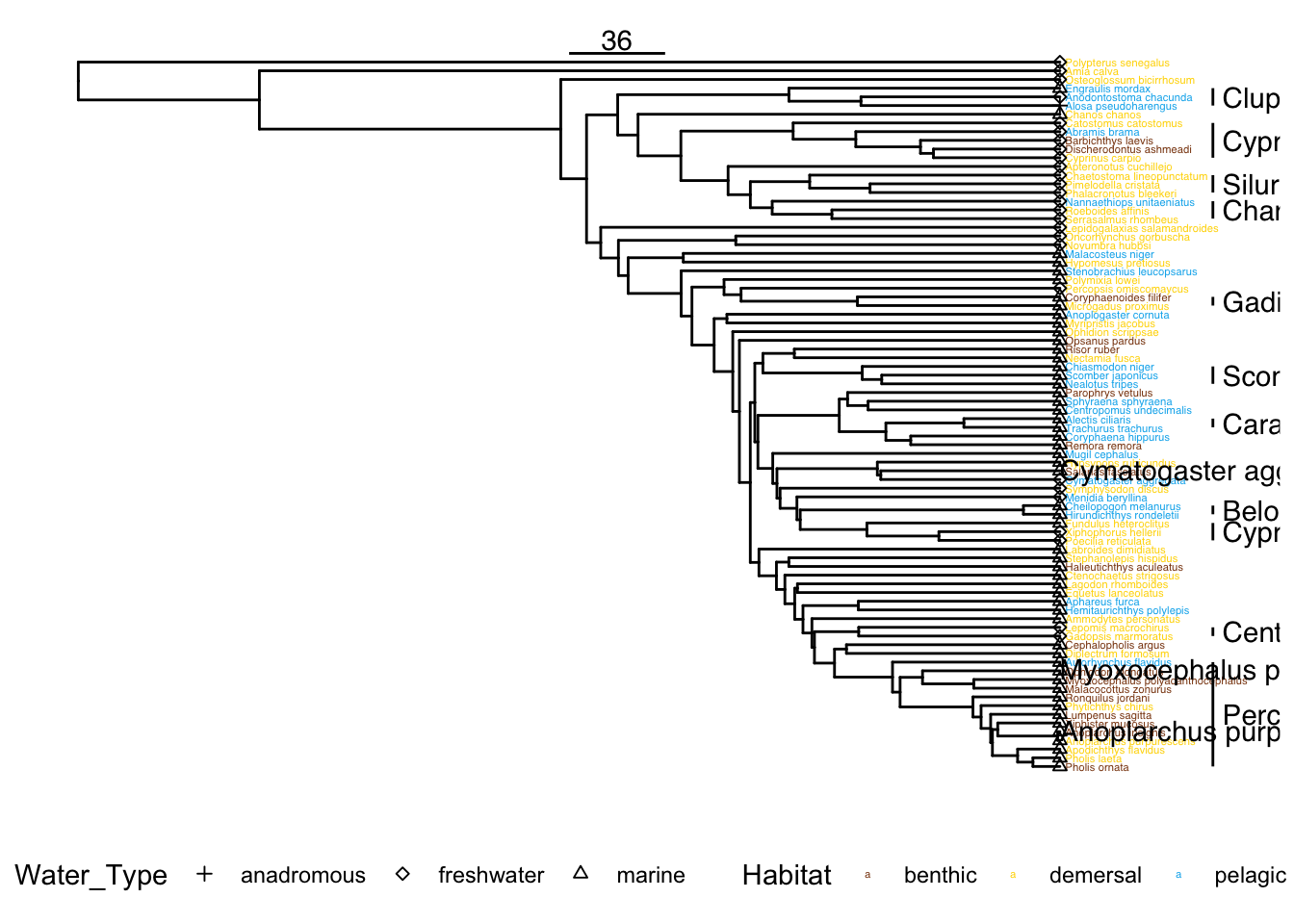
#geom_label2(aes(label='P', subset = ispair))ltt.coplot(verttree, show.tip.label = FALSE)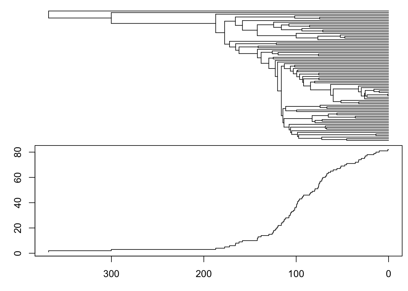
# ggsave(here('output/phylogeny_families.pdf'), width=6.5, height=8, units="in")

ggsave(here('output/plot_example_data_figure.pdf'), width=3.5, height=6, units="in")
vertdata %>%
group_by(Habitat) %>%
summarize(n = n(), frac = n() / nrow(vertdata))# A tibble: 3 × 3
Habitat n frac
<chr> <int> <dbl>
1 benthic 18 0.220
2 demersal 40 0.488
3 pelagic 24 0.293vertdata %>%
group_by(Water_Type) %>%
summarize(n = n(), frac = n() / nrow(vertdata))# A tibble: 3 × 3
Water_Type n frac
<chr> <int> <dbl>
1 anadromous 1 0.0122
2 freshwater 27 0.329
3 marine 54 0.659
sessionInfo()R version 4.2.0 (2022-04-22)
Platform: x86_64-apple-darwin17.0 (64-bit)
Running under: macOS Big Sur/Monterey 10.16
Matrix products: default
BLAS: /Library/Frameworks/R.framework/Versions/4.2/Resources/lib/libRblas.0.dylib
LAPACK: /Library/Frameworks/R.framework/Versions/4.2/Resources/lib/libRlapack.dylib
locale:
[1] en_US.UTF-8/en_US.UTF-8/en_US.UTF-8/C/en_US.UTF-8/en_US.UTF-8
attached base packages:
[1] stats graphics grDevices utils datasets methods base
other attached packages:
[1] plotly_4.10.0 ggtree_3.4.2 here_1.0.1 patchwork_1.1.2
[5] phytools_1.2-0 maps_3.4.0 ape_5.6-2 ggbeeswarm_0.6.0
[9] forcats_0.5.2 stringr_1.4.1 dplyr_1.0.9 purrr_0.3.4
[13] readr_2.1.2 tidyr_1.2.0 tibble_3.1.8 ggplot2_3.3.6
[17] tidyverse_1.3.2
loaded via a namespace (and not attached):
[1] googledrive_2.0.0 colorspace_2.0-3 ellipsis_0.3.2
[4] rprojroot_2.0.3 fs_1.5.2 aplot_0.1.6
[7] rstudioapi_0.14 farver_2.1.1 bit64_4.0.5
[10] optimParallel_1.0-2 fansi_1.0.3 lubridate_1.8.0
[13] xml2_1.3.3 codetools_0.2-18 mnormt_2.1.0
[16] cachem_1.0.6 knitr_1.40 jsonlite_1.8.0
[19] workflowr_1.7.0 broom_1.0.1 dbplyr_2.2.1
[22] compiler_4.2.0 httr_1.4.4 backports_1.4.1
[25] assertthat_0.2.1 Matrix_1.4-1 fastmap_1.1.0
[28] lazyeval_0.2.2 gargle_1.2.0 cli_3.3.0
[31] later_1.3.0 htmltools_0.5.3 tools_4.2.0
[34] igraph_1.3.4 coda_0.19-4 gtable_0.3.1
[37] glue_1.6.2 clusterGeneration_1.3.7 fastmatch_1.1-3
[40] Rcpp_1.0.9 cellranger_1.1.0 jquerylib_0.1.4
[43] vctrs_0.4.1 nlme_3.1-159 crosstalk_1.2.0
[46] xfun_0.32 rvest_1.0.3 lifecycle_1.0.1
[49] phangorn_2.9.0 googlesheets4_1.0.1 MASS_7.3-56
[52] scales_1.2.1 vroom_1.5.7 ragg_1.2.2
[55] hms_1.1.2 promises_1.2.0.1 parallel_4.2.0
[58] expm_0.999-6 yaml_2.3.5 ggfun_0.0.7
[61] yulab.utils_0.0.5 sass_0.4.2 stringi_1.7.8
[64] highr_0.9 plotrix_3.8-2 tidytree_0.4.0
[67] systemfonts_1.0.4 rlang_1.0.4 pkgconfig_2.0.3
[70] evaluate_0.16 lattice_0.20-45 labeling_0.4.2
[73] htmlwidgets_1.5.4 treeio_1.20.2 bit_4.0.4
[76] tidyselect_1.1.2 magrittr_2.0.3 R6_2.5.1
[79] generics_0.1.3 combinat_0.0-8 DBI_1.1.3
[82] pillar_1.8.1 haven_2.5.1 whisker_0.4
[85] withr_2.5.0 scatterplot3d_0.3-41 modelr_0.1.9
[88] crayon_1.5.1 utf8_1.2.2 tzdb_0.3.0
[91] rmarkdown_2.16 grid_4.2.0 readxl_1.4.1
[94] data.table_1.14.2 git2r_0.30.1 reprex_2.0.2
[97] digest_0.6.29 httpuv_1.6.5 numDeriv_2016.8-1.1
[100] textshaping_0.3.6 gridGraphics_0.5-1 munsell_0.5.0
[103] viridisLite_0.4.1 beeswarm_0.4.0 ggplotify_0.1.0
[106] vipor_0.4.5 bslib_0.4.0 quadprog_1.5-8