Summarize vertebral measurements
Last updated: 2022-04-11
Checks: 7 0
Knit directory: Code/
This reproducible R Markdown analysis was created with workflowr (version 1.7.0). The Checks tab describes the reproducibility checks that were applied when the results were created. The Past versions tab lists the development history.
Great! Since the R Markdown file has been committed to the Git repository, you know the exact version of the code that produced these results.
Great job! The global environment was empty. Objects defined in the global environment can affect the analysis in your R Markdown file in unknown ways. For reproduciblity it’s best to always run the code in an empty environment.
The command set.seed(20211230) was run prior to running the code in the R Markdown file. Setting a seed ensures that any results that rely on randomness, e.g. subsampling or permutations, are reproducible.
Great job! Recording the operating system, R version, and package versions is critical for reproducibility.
Nice! There were no cached chunks for this analysis, so you can be confident that you successfully produced the results during this run.
Great job! Using relative paths to the files within your workflowr project makes it easier to run your code on other machines.
Great! You are using Git for version control. Tracking code development and connecting the code version to the results is critical for reproducibility.
The results in this page were generated with repository version e47dde2. See the Past versions tab to see a history of the changes made to the R Markdown and HTML files.
Note that you need to be careful to ensure that all relevant files for the analysis have been committed to Git prior to generating the results (you can use wflow_publish or wflow_git_commit). workflowr only checks the R Markdown file, but you know if there are other scripts or data files that it depends on. Below is the status of the Git repository when the results were generated:
Ignored files:
    Ignored:    .DS_Store
    Ignored:    .Rhistory
    Ignored:    .Rproj.user/
    Ignored:    Flexibility Comparisons.nb.html
    Ignored:    Main.nb.html
    Ignored:    PGLS.FullData.nb.html
    Ignored:    PGLSforeachMeasFeature.nb.html
    Ignored:    PGLSwithPCA_Dims.nb.html
    Ignored:    PreppedVertMeas.nb.html
    Ignored:    ProcessCymatogasterFiles.nb.html
    Ignored:    ProcessFCSVfiles.nb.html
    Ignored:    TestingHabitatwithFriedmanData.nb.html
    Ignored:    Trilok_tree.nb.html
    Ignored:    VertLM.nb.html
    Ignored:    VertMeasLDA_Attempt.nb.html
    Ignored:    VertPGLS.nb.html
    Ignored:    VertPairs.nb.html
    Ignored:    analysis/.DS_Store
    Ignored:    analysis/10-VertLM.nb.html
    Ignored:    analysis/20-plot_phylogeny.nb.html
    Ignored:    analysis/21-plot_fits_and_summary.nb.html
    Ignored:    analysis/CheckSpeciesMatch.nb.html
    Ignored:    caper_test.nb.html
    Ignored:    data/.DS_Store
    Ignored:    ggtree_attempt.nb.html
    Ignored:    plot_example_data.nb.html
    Ignored:    plot_fits_and_summary.nb.html
    Ignored:    plot_phylogeny.nb.html
    Ignored:    renv/library/
    Ignored:    renv/staging/
    Ignored:    summarize_vert_meas.nb.html
    Ignored:    test_phylogeny.nb.html
    Ignored:    test_vertebraspace.nb.html
    Ignored:    vert_evol.Rproj

Untracked files:
    Untracked:  Main.html
    Untracked:  ProcessFCSVfiles.Rmd
    Untracked:  VertPGLS.html
    Untracked:  gg_saver.R
    Untracked:  output/BodyDistribution.pdf
    Untracked:  output/MasterVert_Measurements.csv
    Untracked:  output/mean_d_alphaPos_CBL.pdf
    Untracked:  output/pair_plot.pdf
    Untracked:  output/plot_example_data_figure.pdf
    Untracked:  output/stats_table.rtf
    Untracked:  plot_fits_and_summary.Rmd
    Untracked:  summarize_vert_meas.html
    Untracked:  testtree.csv
    Untracked:  vert_tree.csv
Note that any generated files, e.g. HTML, png, CSS, etc., are not included in this status report because it is ok for generated content to have uncommitted changes.
These are the previous versions of the repository in which changes were made to the R Markdown (analysis/03-summarize_vert_meas.Rmd) and HTML (docs/03-summarize_vert_meas.html) files. If you’ve configured a remote Git repository (see ?wflow_git_remote), click on the hyperlinks in the table below to view the files as they were in that past version.
| File | Version | Author | Date | Message |
|---|---|---|---|---|
| Rmd | 23908bd | Eric Tytell | 2021-12-30 | Test site build again |
| Rmd | edeae3c | Eric Tytell | 2021-12-30 | Rename notebooks to indicate order |
library(tidyverse)── Attaching packages ─────────────────────────────────────── tidyverse 1.3.1 ──✓ ggplot2 3.3.5 ✓ purrr 0.3.4
✓ tibble 3.1.4 ✓ dplyr 1.0.7
✓ tidyr 1.1.3 ✓ stringr 1.4.0
✓ readr 2.0.1 ✓ forcats 0.5.1── Conflicts ────────────────────────────────────────── tidyverse_conflicts() ──
x dplyr::filter() masks stats::filter()
x dplyr::lag() masks stats::lag()library(emmeans)
library(ggbeeswarm)
library(patchwork)
library(here)here() starts at /Users/etytel01/Documents/Vertebrae/CodeLoad data
Vertebral measurements
vertdata <- read_csv(here('output', "MasterVert_Measurements_Matched.csv")) %>%
  separate(MatchSpecies, into=c("MatchGenus", "MatchSpecies"), sep="_") %>%
  relocate(MatchGenus, MatchSpecies, .after=Species) %>%
  rename(alphaPos = alpha_Pos,
         alphaAnt = alpha_Ant,
         DPos = D_Pos,
         DAnt = D_Ant,
         BodyShape = `Body Shape`,
         dBW = d_BW,
         DAntBW = D_Ant_BW,
         DPosBW = D_Pos_BW,
         fineness = `SL/Max_BW`)
Rows: 585 Columns: 54── Column specification ────────────────────────────────────────────────────────
Delimiter: ","
chr (16): Species, Family, Body Shape, Habitat_Initial, Habitat_Friedman, Ha...
dbl (38): Indiv, Pos, SL, CBL_raw, alpha_Pos_raw, d_raw, D_Pos_raw, alpha_An...
ℹ Use `spec()` to retrieve the full column specification for this data.
ℹ Specify the column types or set `show_col_types = FALSE` to quiet this message.head(vertdata)# A tibble: 6 × 55
Species MatchGenus MatchSpecies Family Indiv Pos SL CBL_raw alpha_Pos_raw
<chr> <chr> <chr> <chr> <dbl> <dbl> <dbl> <dbl> <dbl>
1 Alecti… Alectis ciliaris <NA> 1 40 799 24.9 1.51
2 Alecti… Alectis ciliaris <NA> 1 50 799 34.4 1.18
3 Alecti… Alectis ciliaris <NA> 1 60 799 35.8 1.38
4 Alecti… Alectis ciliaris <NA> 1 70 799 36.6 1.34
5 Alecti… Alectis ciliaris <NA> 1 80 799 35.2 1.32
6 Alecti… Alectis ciliaris <NA> 1 90 799 32.8 1.31
# … with 46 more variables: d_raw <dbl>, D_Pos_raw <dbl>, alpha_Ant_raw <dbl>,
# D_Ant_raw <dbl>, CBL <dbl>, alphaPos <dbl>, d <dbl>, DPos <dbl>,
# alphaAnt <dbl>, DAnt <dbl>, Pt1x <dbl>, Pt1y <dbl>, Pt2x <dbl>, Pt2y <dbl>,
# Pt3x <dbl>, Pt3y <dbl>, Pt4x <dbl>, Pt4y <dbl>, Pt5x <dbl>, Pt5y <dbl>,
# Pt6x <dbl>, Pt6y <dbl>, Pt7x <dbl>, Pt7y <dbl>, BodyShape <chr>,
# Habitat_Initial <chr>, Habitat_Friedman <chr>, Habitat_FishBase <chr>,
# Habitat <chr>, Water_Type <chr>, Max_BW_mm <dbl>, BW_slide <dbl>, …Compute the correct CBL
vertdata <-
  vertdata %>%
  rename(CBL_old_raw = CBL_raw,
         CBL_old = CBL) %>%
  mutate(CBL_raw = (abs(Pt1x - Pt3x) + abs(Pt2x - Pt4x))/2,
         CBL = CBL_raw / SL)
ggplot(vertdata, aes(x = CBL_old, y = CBL)) +
geom_point()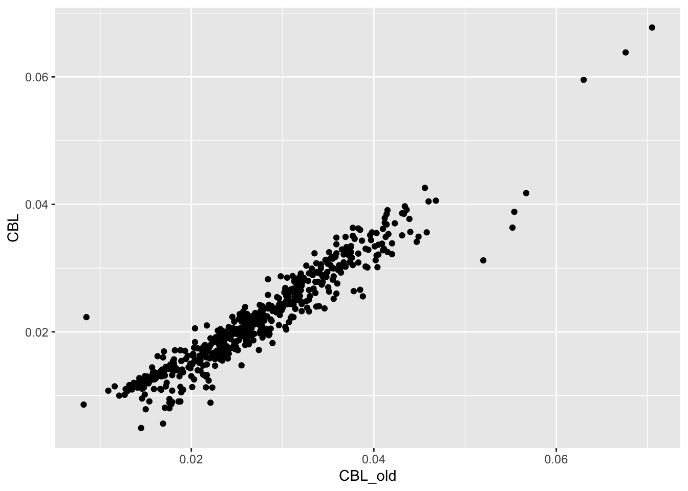 The values are similar but not identical.
Basic plots
vertdata <-
  vertdata %>%
  mutate(d_normD = d / ((DAnt + DPos)/2),
         d_normCBL = d / CBL,
         Iratio = 1 - d^4/((DAnt + DPos)/2)^4) %>%
  mutate(Pos = Pos/100,
         Pos = factor(Pos))
Calculate the mean of each variable at each body position.
vertdata_bypos <-
  vertdata %>%
  group_by(Pos) %>%
  dplyr::summarize(across(c(d, CBL, alphaAnt, alphaPos, DAnt, DPos, dBW, DPosBW, DAntBW,
                            d_normCBL, d_normD, Iratio),
                   list(mn = ~ mean(.x, na.rm = TRUE),
                        med = ~ median(.x, na.rm = TRUE),
                        iqr = ~ IQR(.x, na.rm = TRUE),
                        sd = ~ sd(.x, na.rm = TRUE))))
vertdata_bypos %>%
pivot_longer(!Pos, names_to=c("var", ".value"),
names_pattern = "(.*)_(.*)") %>%
arrange(var, Pos) %>%
ggplot(aes(x = Pos, y = med, group = 1)) +
geom_ribbon(aes(ymin = med-iqr, ymax = med+iqr), alpha = 0.5) +
geom_line() +
geom_line(aes(y = mn), color="red") +
facet_wrap(~ var, scales = "free")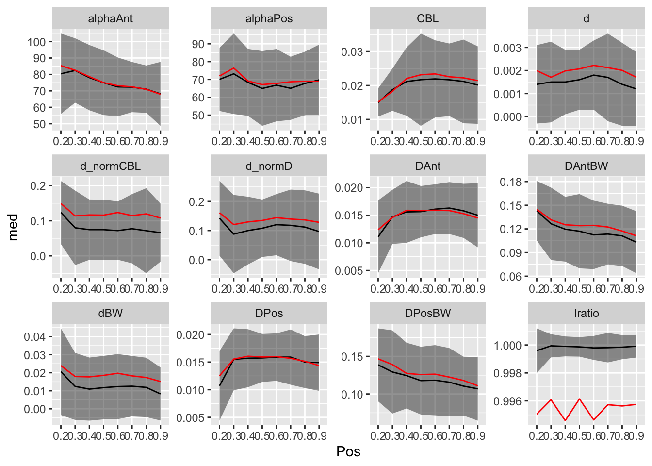
vertdata <-
  vertdata %>%
  group_by(Pos) %>%
  mutate(across(c(d, CBL, alphaAnt, alphaPos, DAnt, DPos, dBW, DAntBW, DPosBW, d_normD, d_normCBL, Iratio),
                   list(ctr = ~.x - median(.x, na.rm = TRUE)))) %>%
  ungroup()
vertdata %>%
ggplot(aes(x = Pos, y = d_ctr, color=Habitat)) +
geom_boxplot(aes(group = Pos)) +
geom_beeswarm() +
geom_line(data = filter(vertdata, d > 0.006 & Habitat == "pelagic"),
aes(group=Species, linetype=Species)) +
geom_label(data = filter(vertdata, d > 0.006 & Pos == 0.9 & Habitat == "pelagic"),
aes(label = Species)) +
facet_grid(. ~ Habitat) +
labs(x = "Vertebra position (L)",
y = "Foramen diameter (L)")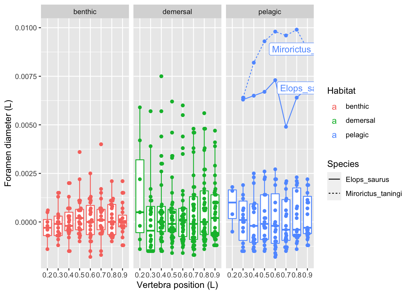
vertdata %>%
  ggplot(aes(x = Pos, y = dBW_ctr, color=Habitat)) +
  geom_boxplot(aes(group = Pos)) +
  geom_beeswarm() +
  geom_line(data = filter(vertdata, dBW_ctr > 0.05 & Habitat == "pelagic"),
             aes(group=Species, linetype=Species)) +
  geom_label(data = filter(vertdata, dBW_ctr > 0.05 & Pos == 0.9 & Habitat == "pelagic"),
              aes(label = Species)) +
  facet_grid(. ~ Habitat) +
  labs(x = "Vertebra position (L)",
       y = "Foramen diameter (L)")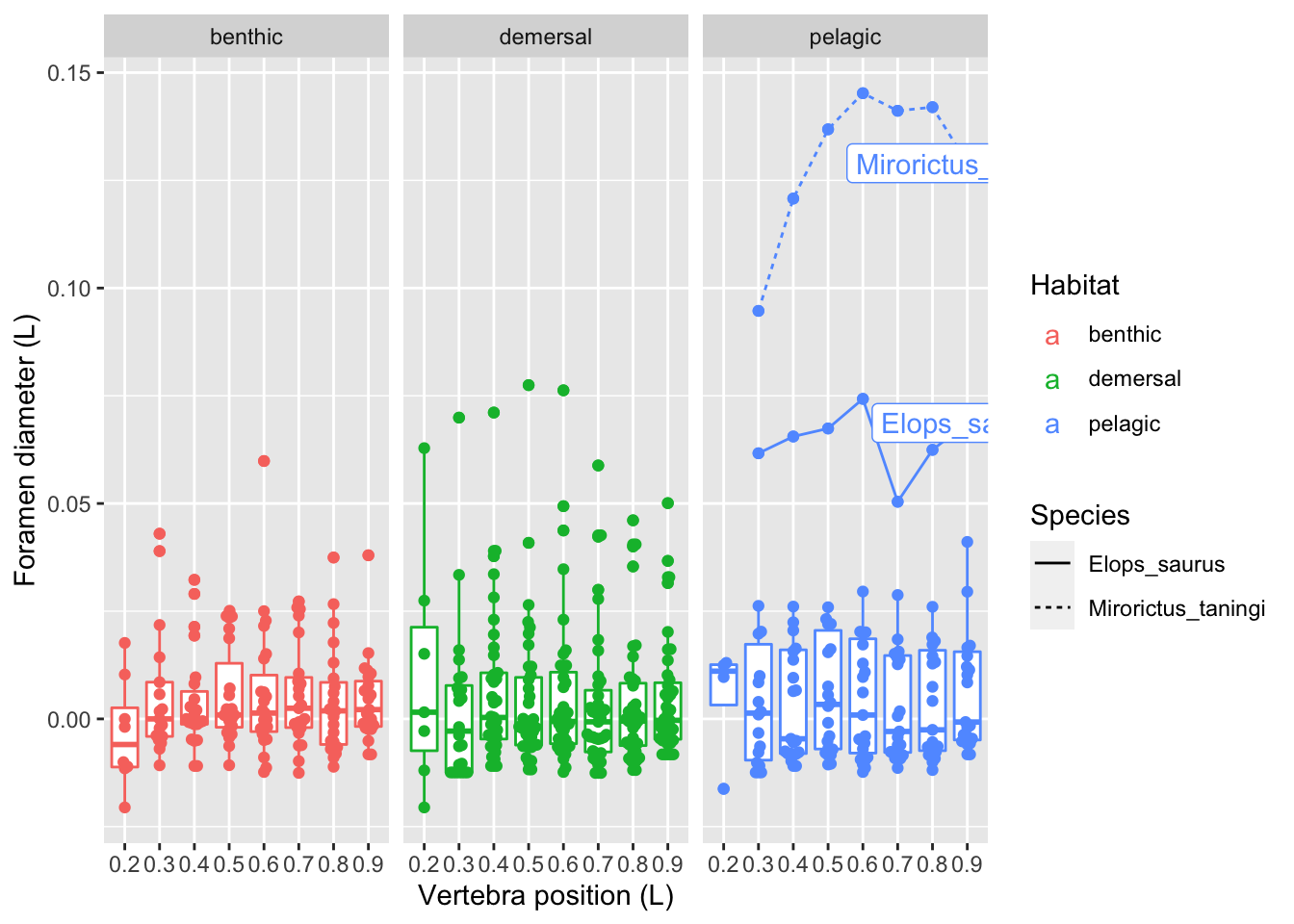
Let’s exclude Elops and Mirorictus from the rest of the analysis for right now.
vertdata2 <-
  vertdata %>%
  filter((Species != "Elops_saurus") &
           Species != "Mirorictus_taningi")
vertdata2 %>%
filter(is.na(d_normCBL))# A tibble: 0 × 71
# … with 71 variables: Species <chr>, MatchGenus <chr>, MatchSpecies <chr>,
# Family <chr>, Indiv <dbl>, Pos <fct>, SL <dbl>, CBL_old_raw <dbl>,
# alpha_Pos_raw <dbl>, d_raw <dbl>, D_Pos_raw <dbl>, alpha_Ant_raw <dbl>,
# D_Ant_raw <dbl>, CBL_old <dbl>, alphaPos <dbl>, d <dbl>, DPos <dbl>,
# alphaAnt <dbl>, DAnt <dbl>, Pt1x <dbl>, Pt1y <dbl>, Pt2x <dbl>, Pt2y <dbl>,
# Pt3x <dbl>, Pt3y <dbl>, Pt4x <dbl>, Pt4y <dbl>, Pt5x <dbl>, Pt5y <dbl>,
# Pt6x <dbl>, Pt6y <dbl>, Pt7x <dbl>, Pt7y <dbl>, BodyShape <chr>, …write_csv(vertdata2, here('output', "vertdata_centered.csv"))plot_position_habitat_distribution <- function(df, var)
{
var <- enquo(var)
p1 <-
df %>%
filter(!is.na(!!var)) %>%
ggplot(aes(x = Pos, y = !!var, color=Habitat, fill=Habitat, group=Habitat)) +
stat_summary(fun.data = "mean_se", geom="ribbon", alpha=0.5) +
stat_summary(fun = "mean", geom="line")
p2 <-
df %>%
filter(!is.na(!!var)) %>%
ggplot(aes(x = Habitat, y = !!var, color=Habitat)) +
geom_violin() +
geom_boxplot(width=0.3, alpha=0.5) +
stat_summary(aes(group = 1), fun = "median", geom = "line")
p1 + p2 + plot_layout(widths = c(3,1), guides = 'collect')
}plot_position_habitat_distribution(vertdata2, d)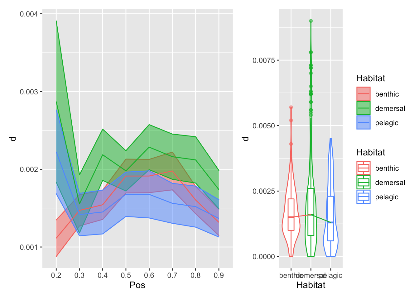 Here we’re plotting the foramen diameter (normalized by body length) relative to position on the left, and the overall distributions relative to habitat on the right. The bottom row has the overall mean pattern relative to body length subtracted.
plot_position_habitat_distribution(vertdata2, dBW)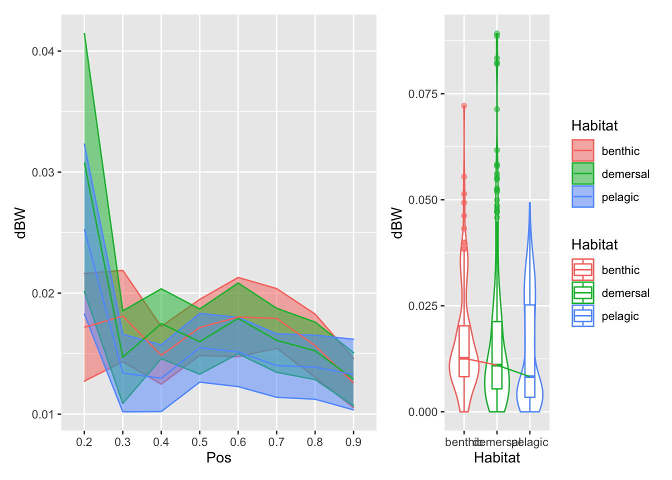
plot_position_habitat_distribution(vertdata2, CBL)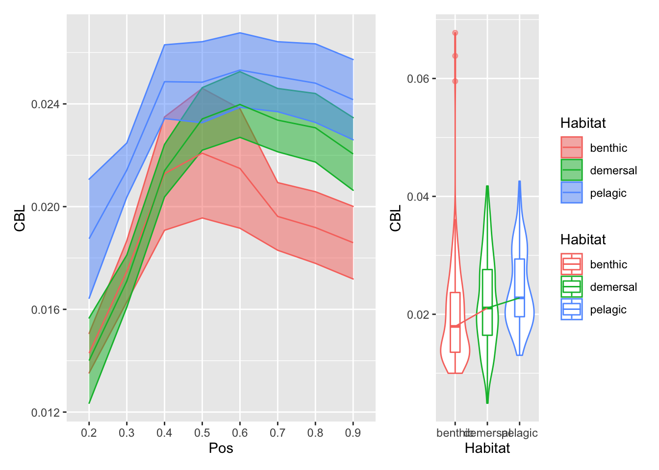
plot_position_habitat_distribution(vertdata2, alphaAnt)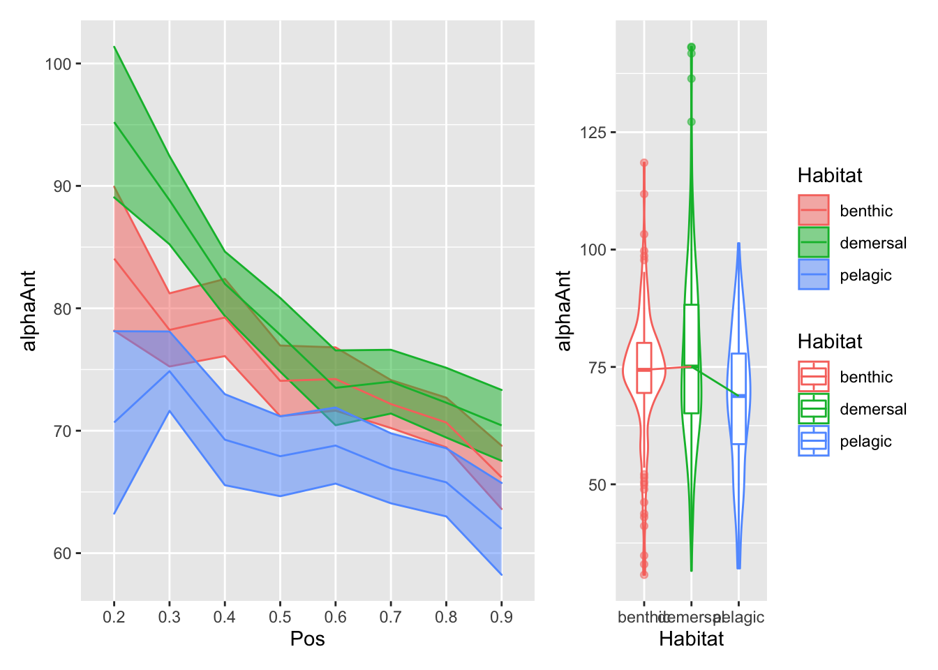
plot_position_habitat_distribution(vertdata2, alphaPos)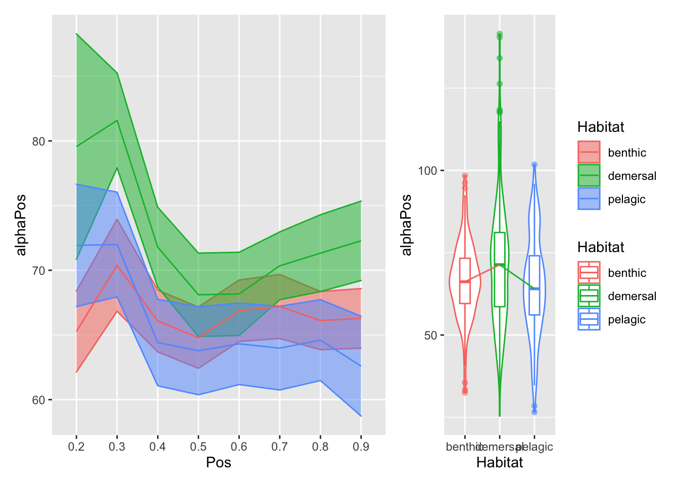
plot_position_habitat_distribution(vertdata2, DAnt)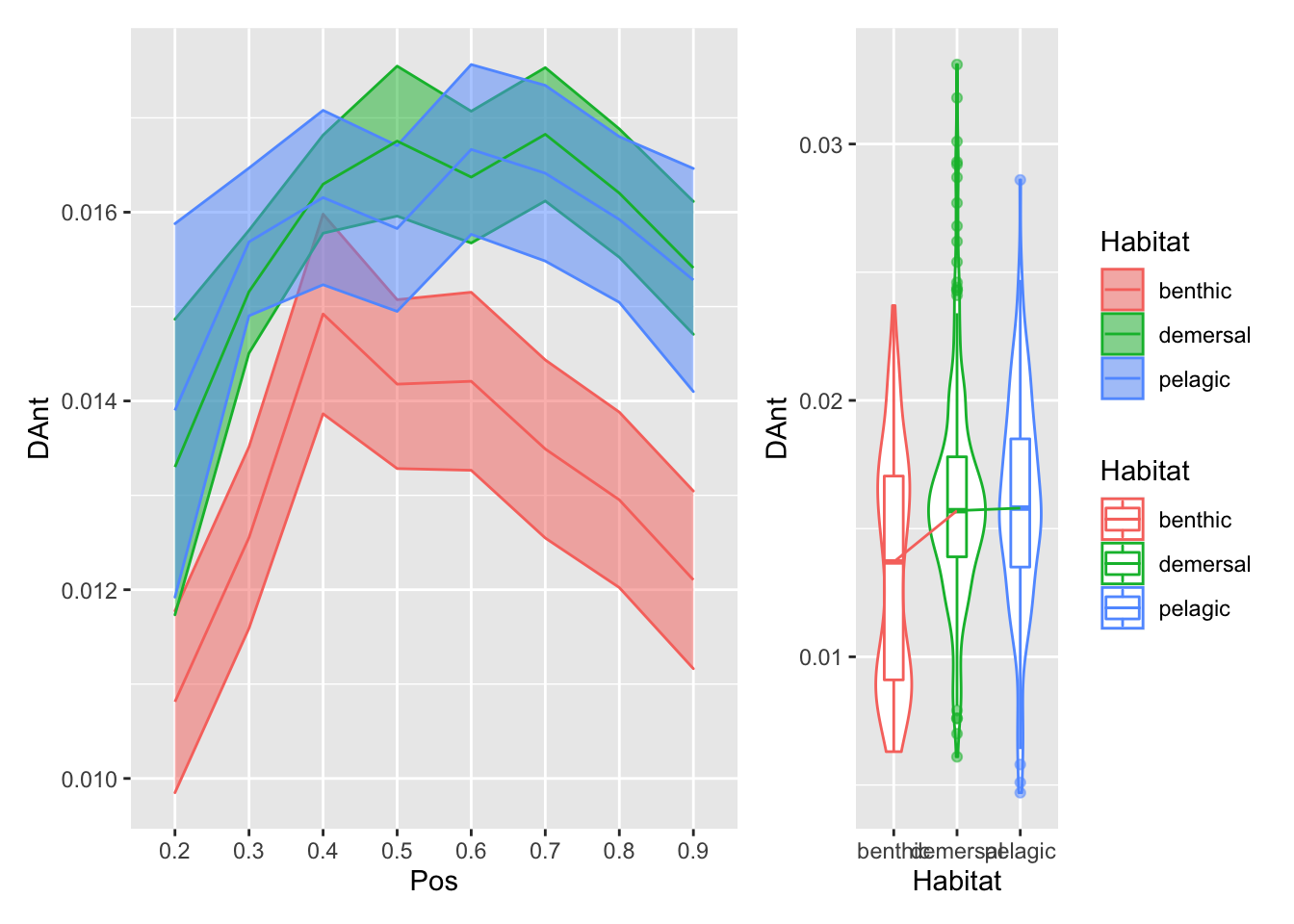
Compare summary statistics
First generate the summary statistics, summarizing across the body positions.
This gives us the mean, median, and max values for each of the measurements.
vertdata_summary <-
  vertdata2 %>%
  filter(Pos != 0.2 & Pos != 0.3) %>%
  group_by(Species, Indiv, Habitat, Water_Type, MatchSpecies, MatchGenus, fineness) %>%
  dplyr::summarize(across(c(CBL, d, alphaAnt, alphaPos, DAnt, DPos,
                     dBW, DAntBW, DPosBW, d_normCBL, d_normD, Iratio),
                   list(med = ~ median(.x, na.rm = TRUE),
                        max = ~ max(.x, na.rm = TRUE),
                        mn = ~ mean(.x, na.rm = TRUE)))) %>%
  ungroup()
`summarise()` has grouped output by 'Species', 'Indiv', 'Habitat', 'Water_Type', 'MatchSpecies', 'MatchGenus'. You can override using the `.groups` argument.head(vertdata_summary)# A tibble: 6 × 43
Species Indiv Habitat Water_Type MatchSpecies MatchGenus fineness CBL_med
<chr> <dbl> <chr> <chr> <chr> <chr> <dbl> <dbl>
1 Abramis_bra… 1 pelagic freshwater alburnus Alburnus 8.95 0.0166
2 Alectis_cil… 1 demers… marine ciliaris Alectis 8.75 0.0346
3 Alosa_pseud… 1 pelagic anadromous pseudoharen… Alosa 7.39 0.0165
4 Amia_calva 1 demers… freshwater calva Amia 6.72 0.00983
5 Ammodytes_p… 1 benthic marine dubius Ammodytes 16.9 0.0132
6 Anodontosto… 1 pelagic freshwater cepedianum Dorosoma 4.66 0.0228
# … with 35 more variables: CBL_max <dbl>, CBL_mn <dbl>, d_med <dbl>,
# d_max <dbl>, d_mn <dbl>, alphaAnt_med <dbl>, alphaAnt_max <dbl>,
# alphaAnt_mn <dbl>, alphaPos_med <dbl>, alphaPos_max <dbl>,
# alphaPos_mn <dbl>, DAnt_med <dbl>, DAnt_max <dbl>, DAnt_mn <dbl>,
# DPos_med <dbl>, DPos_max <dbl>, DPos_mn <dbl>, dBW_med <dbl>,
# dBW_max <dbl>, dBW_mn <dbl>, DAntBW_med <dbl>, DAntBW_max <dbl>,
# DAntBW_mn <dbl>, DPosBW_med <dbl>, DPosBW_max <dbl>, DPosBW_mn <dbl>, …vertdata_summary %>%
select(ends_with("max") | Habitat | Species) %>%
pivot_longer(contains("max"),
names_to = "var", values_to = "value") %>%
ggplot(aes(x = Habitat, y = value, color = Habitat)) +
geom_violin() +
geom_boxplot(width=0.3, alpha=0.5) +
stat_summary(aes(group = 1), fun = "median", geom = "line") +
facet_wrap(~ var, scales = "free")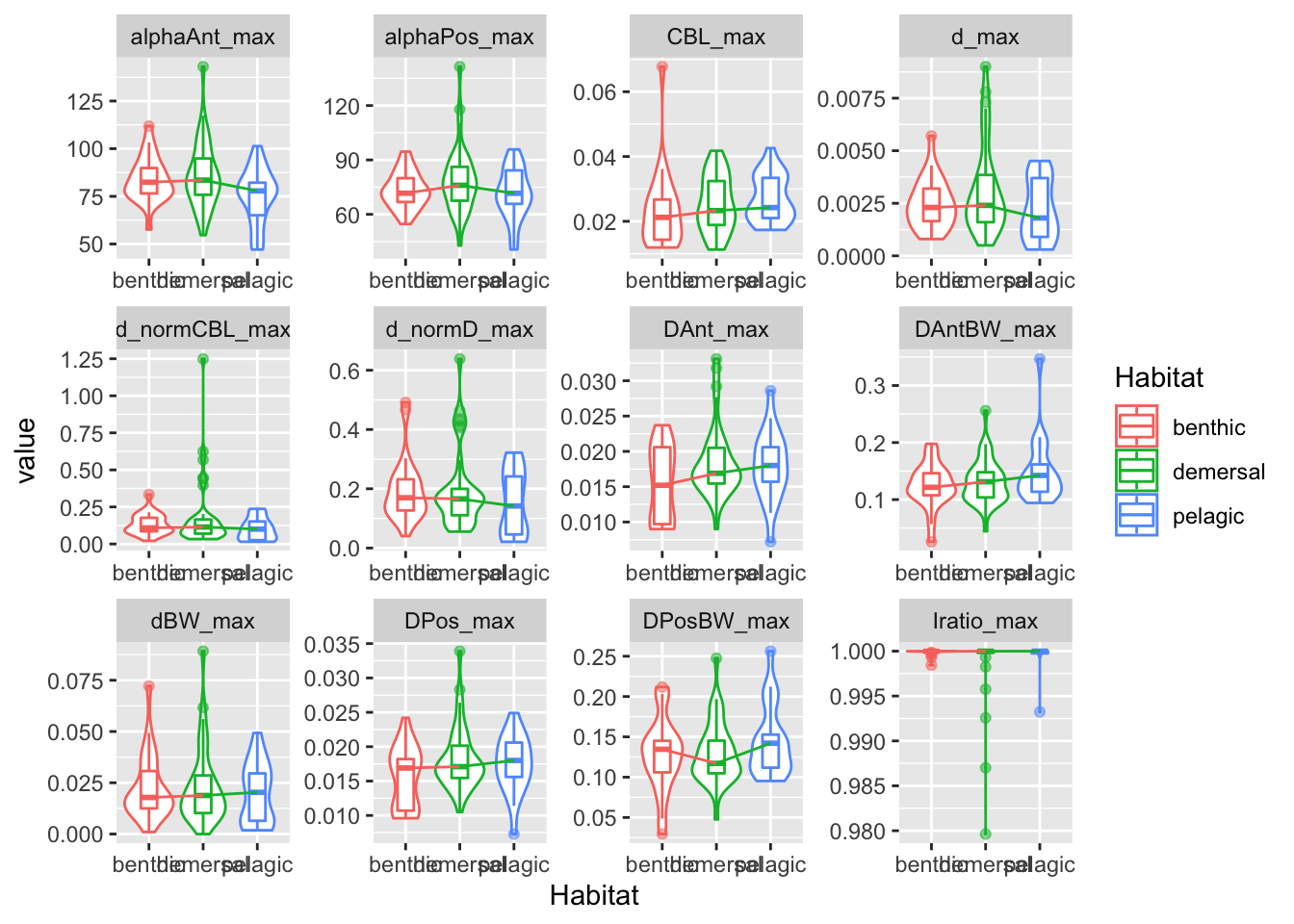
write_csv(vertdata_summary, here("output", "vertdata_summary.csv"))
sessionInfo()R version 4.1.2 (2021-11-01)
Platform: x86_64-apple-darwin17.0 (64-bit)
Running under: macOS Big Sur 10.16
Matrix products: default
BLAS: /Library/Frameworks/R.framework/Versions/4.1/Resources/lib/libRblas.0.dylib
LAPACK: /Library/Frameworks/R.framework/Versions/4.1/Resources/lib/libRlapack.dylib
locale:
[1] en_US.UTF-8/en_US.UTF-8/en_US.UTF-8/C/en_US.UTF-8/en_US.UTF-8
attached base packages:
[1] stats graphics grDevices datasets utils methods base
other attached packages:
[1] here_1.0.1 patchwork_1.1.1 ggbeeswarm_0.6.0 emmeans_1.6.3
[5] forcats_0.5.1 stringr_1.4.0 dplyr_1.0.7 purrr_0.3.4
[9] readr_2.0.1 tidyr_1.1.3 tibble_3.1.4 ggplot2_3.3.5
[13] tidyverse_1.3.1
loaded via a namespace (and not attached):
[1] httr_1.4.2 bit64_4.0.5 vroom_1.5.4 jsonlite_1.7.2
[5] modelr_0.1.8 assertthat_0.2.1 highr_0.9 renv_0.14.0
[9] vipor_0.4.5 cellranger_1.1.0 yaml_2.2.1 pillar_1.6.2
[13] backports_1.2.1 lattice_0.20-45 glue_1.4.2 digest_0.6.27
[17] promises_1.2.0.1 rvest_1.0.1 colorspace_2.0-2 htmltools_0.5.2
[21] httpuv_1.6.4 pkgconfig_2.0.3 broom_0.7.9 haven_2.4.3
[25] xtable_1.8-4 mvtnorm_1.1-2 scales_1.1.1 whisker_0.4
[29] later_1.3.0 tzdb_0.1.2 git2r_0.29.0 farver_2.1.0
[33] generics_0.1.0 ellipsis_0.3.2 withr_2.4.2 cli_3.0.1
[37] magrittr_2.0.1 crayon_1.4.1 readxl_1.3.1 estimability_1.3
[41] evaluate_0.14 fs_1.5.0 fansi_0.5.0 xml2_1.3.2
[45] beeswarm_0.4.0 tools_4.1.2 hms_1.1.0 lifecycle_1.0.0
[49] munsell_0.5.0 reprex_2.0.1 compiler_4.1.2 rlang_0.4.11
[53] grid_4.1.2 rstudioapi_0.13 labeling_0.4.2 rmarkdown_2.10
[57] gtable_0.3.0 DBI_1.1.1 R6_2.5.1 lubridate_1.7.10
[61] knitr_1.34 bit_4.0.4 fastmap_1.1.0 utf8_1.2.2
[65] workflowr_1.7.0 rprojroot_2.0.2 stringi_1.7.4 parallel_4.1.2
[69] Rcpp_1.0.7 vctrs_0.3.8 dbplyr_2.1.1 tidyselect_1.1.1
[73] xfun_0.25 coda_0.19-4